Distributed systems can be represented by communication graphs, composed of two elements: vertices and edges. Vertices represent processes or nodes and edges represent direct communication channels between two vertices. If the communication channel is one-way, i.e. only from vertex i to vertex j without the way back, edges are oriented and the graph is called a directed graph. However, this thesis assumes only bidirectional communication channels, i.e. unoriented edges in undirected graphs.
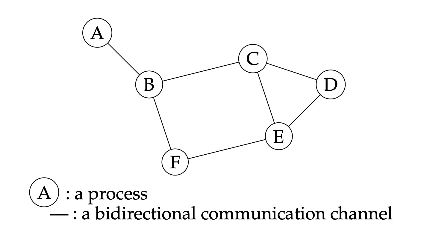
Two processes connected with a channel are called neighbors, such as process i is a neighbor of process j if they there is a direct edge between them. The set of processes connected to process i is called the neighborhood of i. For example, considering 2.6, process A is a neighbor of process B, and the neighborhood of process B is the set of processes {A,C,F}.
Neighbors of a process have a communication distance of one hop, and are called 1-hop neighbors, as they can directly communicate with it. Neighbors of neighbors of a process are at a distance of 2-hop of this process, and so on. When the distance is higher than one, the term multi-hop can be used. The hop count distance refers to the number of processes between two processes. For example, considering 2.6, process B is a 1-hop neighbor of process A, and process E is a 3-hop neighbor of process A.
As processes are autonomous entities, when a process needs to communicate with a process located further than 1-hop, intermediate processes located between the sender and the final receiver, are called relays and act as routers, establishing a path from the sender to the destination process over which the message is transmitted.
Different assumptions about network knowledge can be made: known networks, where nodes have a knowledge of the system, and unknown networks, with the weakest possible assumptions about knowledge, communication graph, channel connectivity and reliability, in order to be as close as possible to reality.
There are two main types of networks: static and dynamic networks.
Originally, distributed systems were based on static networks. A static system is composed of a finite set of nodes, where the membership of the system can only change because of failures. The communication graph is static during the execution of the system, however, network partitions can arise due to failures. Nodes do not move, nor leave, neither join the system.
As an example, the links of a static system can physically be either wires between nodes, or wireless radio wave antennas with a fixed transmission range.
With the advent of peer-to-peer technologies and mobile devices such as mobile phones, mobile sensors, autonomous vehicular or drones, nodes of a network are able to move, join, or leave the system. They can also fail. Therefore, the membership of the system is no longer finite but may vary over time. Communication channels between nodes are non-persistent and can also change over time, which may lead to network partitions.
There is no unique definition of dynamic systems in the literature [Agu04; KLO10; BRS12; Lar+12]. Some authors define it as a distributed system where the communication graph evolves over time. Others give the definition of a model where nodes join and leave the system at arbitrary times during the system execution.
Dynamic systems can be represented by a dynamic communication graph. Many works characterize the dynamics of graphs, such as the Time-Varying Graph (TVG) proposed by Casteigts et al. [Cas+11] (where relations between nodes take place over a time span 𝒯 , with a presence function indicating whether a given edge is available at a given time), Flocchini et al. [FMS09] and Tang et al. [Tan+10], evolving graphs by Ferreira [Fer04], temporal network by Kempe et al. [KKK02], graphs over time by Leskovec et al. [LKF07], or temporal graph by Kostakos [Kos09].
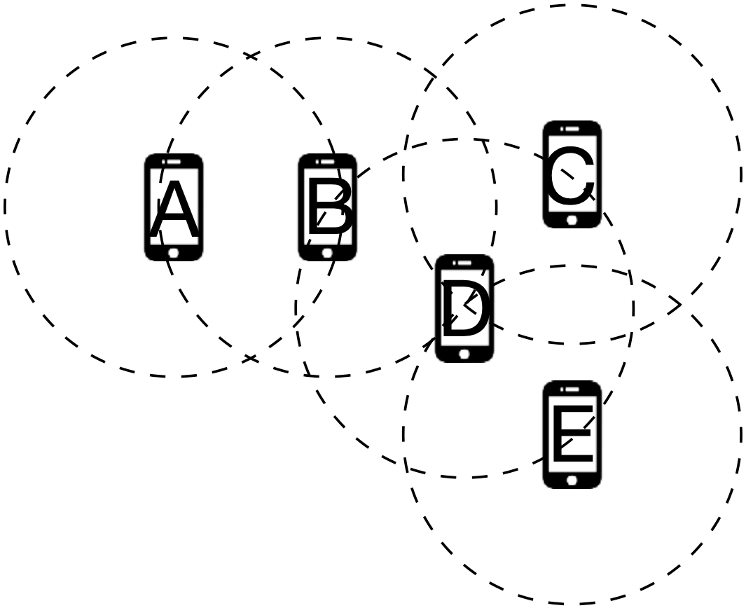
Physically, the links of a dynamic system can be, for example, wireless communication with radio wave antennas. A representation of a dynamic network is given in 2.7.