Some preliminary results about the energy consumption of nodes executing Centrality-based Eventual Leader (CEL) and Gómez-Calzado et al. algorithms (Chapter 5) are presented in the following.
Experiments were conducted on the OMNeT++ [VH08]/INET [MVK19] environment described in Section 5.3, with the same configuration. However, the transmission range is fixed between 30 meters (instead of 20 meters) and 80 meters.
The power consumption consumer model for IEEE 802.11 used the following constant parameter values approximately based on a CC3220 transceiver:
Local computation (CPU) and mobility are not considered in the energy consumption model, neither the power transmission range fixed at each experiment. Each experiment lasts 30 simulated minutes.
The two versions of CEL, i.e. CEL-1 and CEL-0.7, and Gómez-Calzado et al. algorithm [Góm+13] are compared using the same settings has in Section 5.3.1.
The two mobility models defined in Section 5.3.2 are used, i.e. Random Walk and Truncated Lévy Walk.
The energy consumption is computed using the radio power consumer model describe in A.1.1, where transmission, reception, or idle states consume energy from the node battery. At the end of each experience, the energy consumption per node for each algorithm is computed and measured in watts (W).
Overall, the energy consumption per node is correlated with the number of messages sent, presented in Section 5.4.2, as the power consumption consumer model considers only communication.
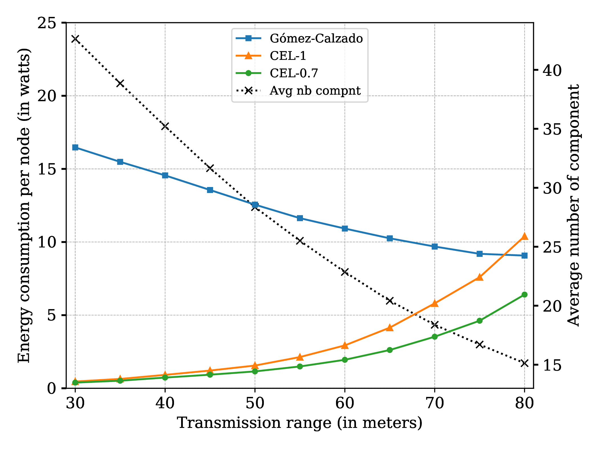
For the Random Walk mobility model in A.1, the power consumption of nodes in the Gómez-Calzado et al. algorithm decreases as the transmission range increases, since more nodes are in the same component and timeouts of leader messages are higher. The power consumption of both versions CEL algorithms increase as the transmission range increase, since movements in larger connected component lead to more messages sent. In lower transmission ranges, the energy consumption per node executing Gómez-Calzado et al. algorithm is higher than both CEL versions. For instance, at a transmission range of 30 meters, nodes executing Gómez-Calzado et al. algorithm consume on average 16.47W, while nodes in CEL-1 and CEL-0.7 consume on average 0.46W and 0.39W respectively. The probabilistic gossip version of CEL with ρ sets to 0.7 reduces the energy consumption compared to CEL-1, since less messages are sent as seen in Section 5.4.2, due to the self-pruning approach used in the TopologicalBroadcast method described in Section 5.2.8. Nodes in CEL-0.7 have an energy consumption of 6.41W on average at a transmission range of 80 meters, while nodes in CEL-1 and Gómez-Calzado et al. algorithms are up to 10.39W and 9.07W respectively.
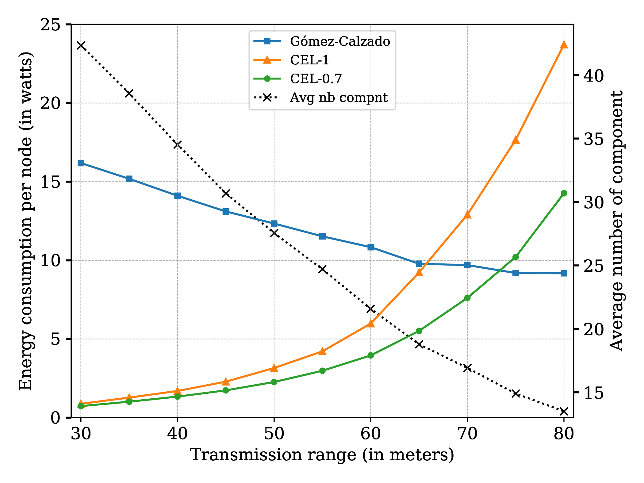
A.2 shows a higher average energy consumption for nodes executing CEL-1 than Gómez-Calzado et al. in the Truncated Lévy Walk mobility model when the transmission range is larger than 65 meters. A similar observation can be made concerning the average number of messages sent on this mobility model as presented in Section 5.4.2. At a transmission range of 80 meters, nodes executing CEL-0.7 have an average energy consumption up to 14.27W, while nodes executing CEL-1 are up to 23.72W, and nodes in Gómez-Calzado et al. algorithm are up to 9.18W. These increase are due to flying nodes that induce many connections and disconnections among existing connected components. However, the energy consumption per node remains lower for both CEL versions than Gómez-Calzado et al. algorithm on smaller ranges such as 30 meters.
Note that this preliminary evaluation is a work in progress.