The objective of the simulations is to compare the Topology Aware algorithm with a flooding one.
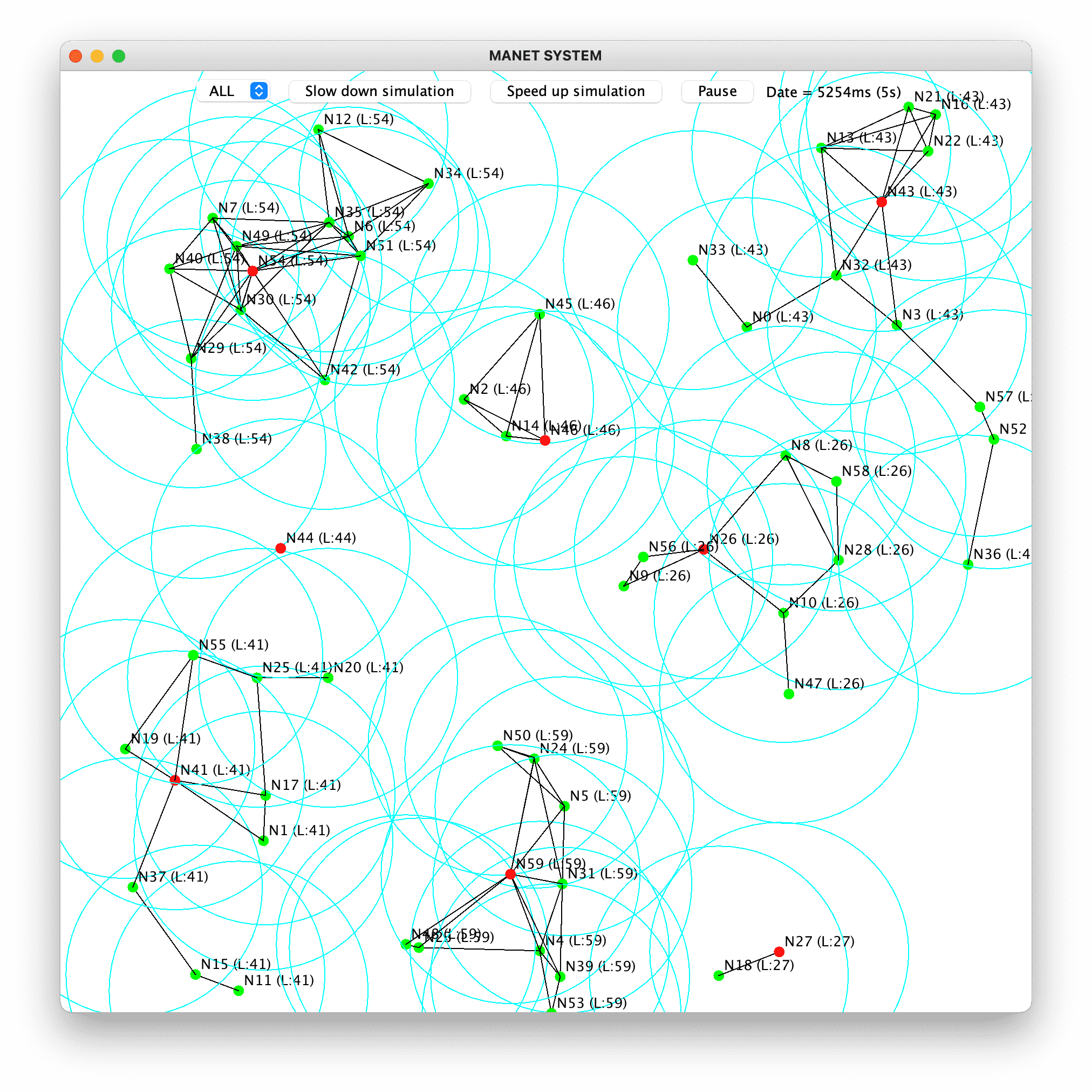
Several evaluation experiments were conducted on PeerSim [MJ09], a Java peer-to-peer network simulator with an event-based engine and modularity. Each experiment lasts 30 minutes, with a simulated unit of time corresponding to one millisecond, and simulates 60 nodes placed in a 900 × 900 meters obstacle-free area, with a fixed diameter of transmission range between 10 and 200 meters decided beforehand and identical for all nodes. Message sending latency follows a Poisson distribution with parameter λ = 10. The experiments were conducted using console-mode on remote servers, but a graphical interface was used primarily for development purposes, as shown in 4.10.
Two versions of the Topolgy Aware algorithm were considered:
These two versions of the Topology Aware algorithm were compared with a variant of the Vasudevan et al. algorithm [VKT04], which is based on flooding. Vasudevan et al. algorithm returns ⊥ during the election phase, if the leader has not been elected yet. In order to be fairly comparable with the Topology Aware algorithm, a variant of this algorithm that never returns ⊥ but a possible current leader, is considered. Indeed, in Topology Aware, a correct node is always able to render a leader according to its topological knowledge. This variant is denoted Flooding because each node periodically broadcasts leader messages informing its current leader to neighbor nodes.
Note that Flooding is also a variant of the OptFloodMax algorithm that Nancy A. Lynch introduced in her book Distributed Systems [Lyn96]. In OptFloodMax, processes send their unique identifier to their neighbors, whenever a process obtains a new maximum unique identifier (which will eventually be elected as the leader).
The Flooding algorithm was adapted for MANET assuming an underlying probe system that detects connections and disconnections. Exchanged leader messages contain the node identifier and an election criterion, called value. The leader is the node with the highest value. It periodically broadcasts leader messages to neighbor nodes every α milliseconds, and each node forwards this information to neighbors. When the leader fails, it stops sending leader messages, and after a non-reception of β leader messages from the leader, nodes trigger a new election by setting themselves as their own new leader. Thus, new leader messages from different nodes are propagated, and eventually, the node with the highest value is elected.
In order to elect a leader with good local connectivity, it is considered that the value is equal to the number of direct neighbors of a node, equivalent to node degree in a graph, which is updated at each topology change, thanks to the probe system (new connection or disconnection). The highest node identifier is used to break ties among identical values. This algorithm is denoted Flooding Degree.
In the Flooding Degree algorithm, nodes send leader messages every α = 250 milliseconds. Every node triggers a new election if β = 1 leader message from the current leader was not received after a timeout of 300 milliseconds.
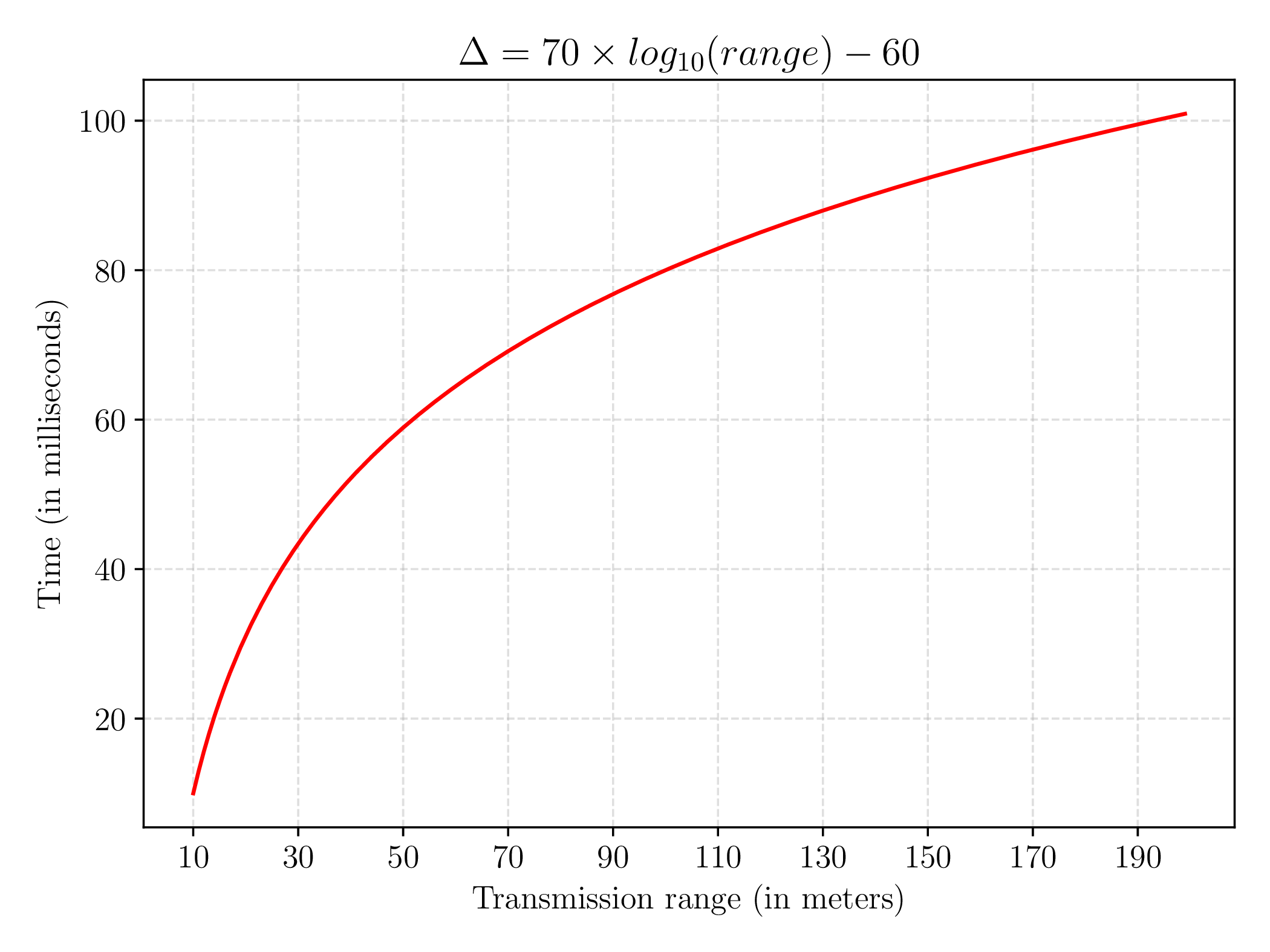
In both Topology Aware versions, updates are kept in a list acting as a buffer, before being sent every Δ milliseconds if the list is not empty. The value of Δ is based on the transmission range (on x-axis of figures), considering that the larger the transmission range, the higher number of nodes potentially reached. Thus, to avoid burst effect after topology changes, the value of Δ should make information transmission faster on small components, but slower on lager components, due to the high dynamics of mobile nodes induced by larger transmission ranges. To this aim, the following formula was deduced empirically:

With this formula, Δ has a low value for small ranges and increases proportionally to the size of the range, with a fast increase for low ranges and a slow increase for higher ranges, as shown in 4.11. Therefore, information is transmitted quickly on small components, but more slowly on larger components. As a result, updates are sent every 60 milliseconds on average for lower transmission ranges, and every 90 milliseconds on average for larger transmission ranges.
In the three algorithms, when a probe message is received by node i, the Connection method of the algorithm is triggered. A probe message contains the unique identifier of the node and is sent every τ = 400 milliseconds. If γ = 1 probe message from node j is not received after a timeout of 450 milliseconds, node i considers node j as out of range and trigger the Disconnection method.
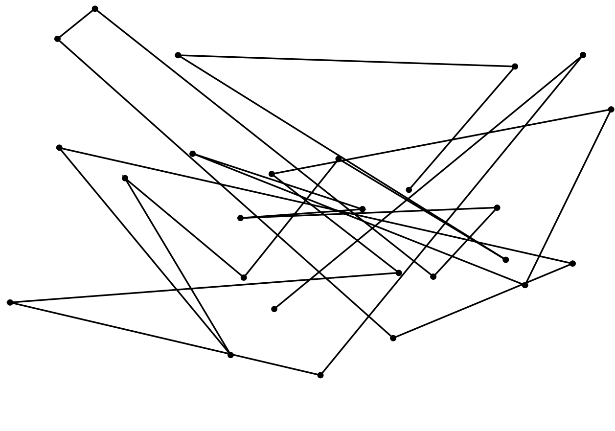
Two different mobility patterns have been considered in the experiments: the random waypoint and a periodic disc positioning pattern around a single point of interest. For both mobility patterns, the minimum node speed is set to 5 m/s and the maximum node speed is set to 15 m/s. The chosen speed follows a uniform distribution between the minimum and the maximum speed.
Nodes are randomly placed in the area and move according to the Random Waypoint mobility model [CBD02]. Nodes wait 10 seconds before choosing the next random destination. It is worth noting that this mobility pattern is largely used in the literature [VKT04; CBD02]. A representation of the Random Waypoint is given in 4.12.
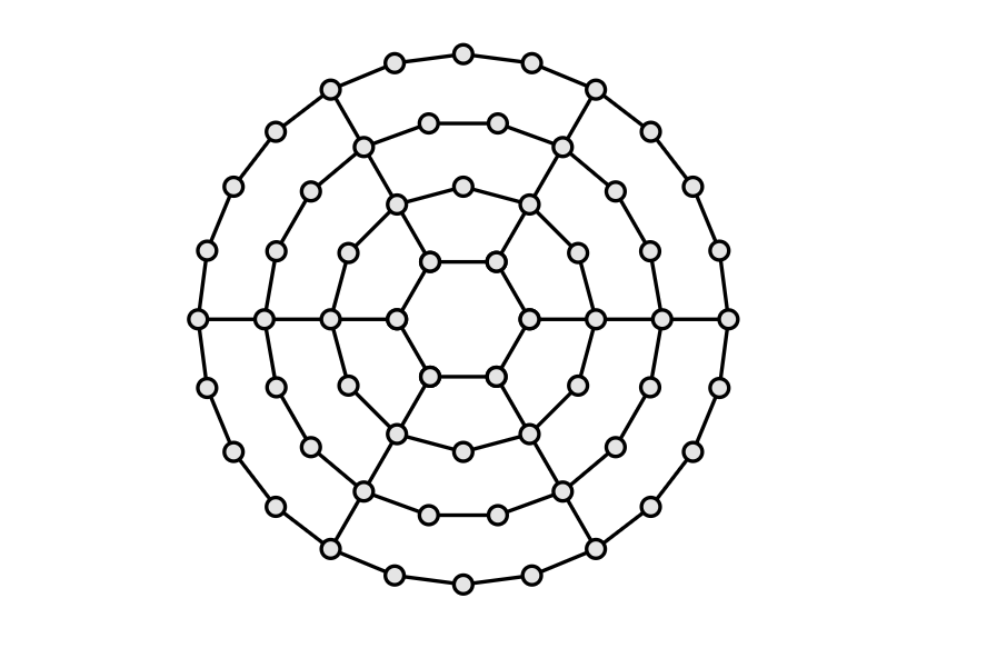
First, nodes are placed to create concentric circles whose center is the same unique point of interest, thus, composing a disc, like the one shown in 4.13, such that there exists a path between any two nodes in the disc.
After 10 seconds, nodes start moving to a randomly chosen destination. Once reached, nodes wait 10 seconds before going back to their initial position in the circle, waiting for each other nodes to reach its initial position. Note that nodes can wait a long time for the other nodes to return to their initial position in the disc, due to various node speeds. When every node is at its initial circle position (the disc is reconstructed again), they wait 10 seconds before moving to another random destination, and repeat this behavior continually until the end of the experiment.
The shape of the disc is independent of the node transmission range, i.e. it always looks like the one in 4.12 regardless of the diameter of the transmission range. This pattern could model user activities, where nodes represent people visiting regularly just a few places [Pap+16].