As processes can take a long time to reply, can fail, or even simply leave the network during execution of the system, the communication between processes is uncertain. To take into account this uncertainty, the literature uses an underlying model that considers:
Three main timing models were defined [Lyn96]:
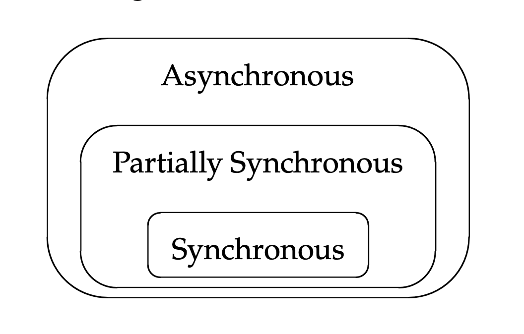
Among these three timing models, synchronous systems are included in partially synchronous systems, which are included in asynchronous systems, as shown in 2.1 [Cam20].
Note that there exist many other intermediate models between the synchronous and asynchronous models.
The different types of temporal models are summarized in 2.1.
| Message latency | Computation time | |
| bound δ | bound ϕ | |
| Synchronous model | Exist, known and finite
| |
| Asynchronous model | Do not exist
| |
| Partially synchronous model | Exist but unknown
| |