5.3 Simulation Environment

Realistic simulations were carried over in order to compare the Centrality-based Eventual Leader (CEL) algorithm, with the Ω eventual leader election algorithm of Gómez-Calzado et al. [Góm⁺13] (see Section 3.2.2).

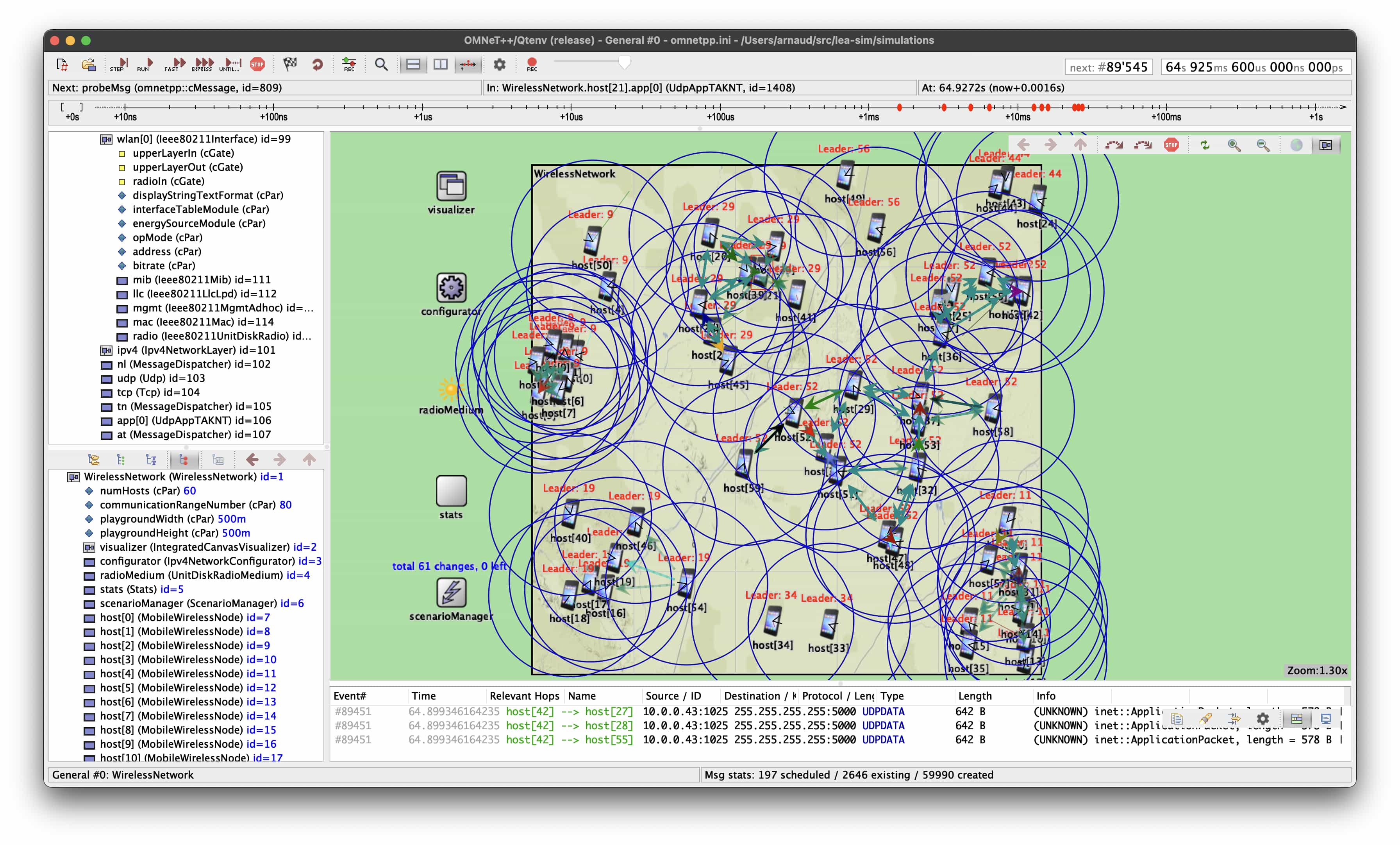
Experiments were conducted on a C++ discrete event simulator called OMNeT++ [VH08], with the INET framework [MVK19] to model wireless protocols and mobile networks. This environment allows simulation of unreliable communication channels and realistic layers of the OSI communication model. Each experiment involves 60 moving nodes placed in a 500 × 500 meters obstacle-free area during 30 simulated minutes. The experiments were conducted using OMNeT++ in console-mode on remote servers, but a graphical interface shown in 5.1 was mainly used for development purposes.

Simulations consider a full MANET network stack, with the physical and data-link layers following the IEEE 802.11n specifications [09]. The use of a cross-layer mechanism at the MAC level allows the application layer to access neighbor’s MAC addresses. Therefore, the identifier of a node is a MAC address, encoded on 3 bytes rather than usually 6 bytes, as it is assumed that all nodes have network components from the same manufacturer. Every node uses a single transceiver, with a fixed transmission range decided at the beginning of the experiment between 20 and 80 meters, and identical for all nodes. This transceiver uses the 2.4 GHz frequency band, with a nominal bitrate of 52 Mbps.

5.3.1 Algorithms Settings

In CEL, beacon messages are sent by the data-link layer every τ = 102.4 milliseconds (usual interval value of the Target Beacon Transmission Time), and are detected at the MAC level by the cross-layer mechanism.

The following two configurations of the algorithm were used for evaluation:

• In CEL-1, the probability ρ to gossip a knowledge message in the TopologicalBroadcast method is set to 1. Therefore, messages are flooded in the network, if the neighborhood of the sender node is different from the receiver’s one.
• In CEL-0.7, ρ is set to 0.7, i.e. a message is retransmitted with 0.7 probability [HHL02], if the sender and receiver neighborhoods are different.

In Gómez-Calzado et al. algorithm, the frequency to send either join messages when a node is unconnected, or leader messages, is 102.4ms, as both are considered beacon messages. The timers detecting leader failure and node disconnection have an initial value (100ms) which is increased by 500ms when they expire. Since the original paper does not give any indication on the parameter values, these values were chosen after running several experiments using different values, as they were the most favorable to Gómez-Calzado et al. algorithm.

5.3.2 Mobility Models

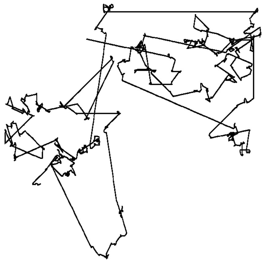
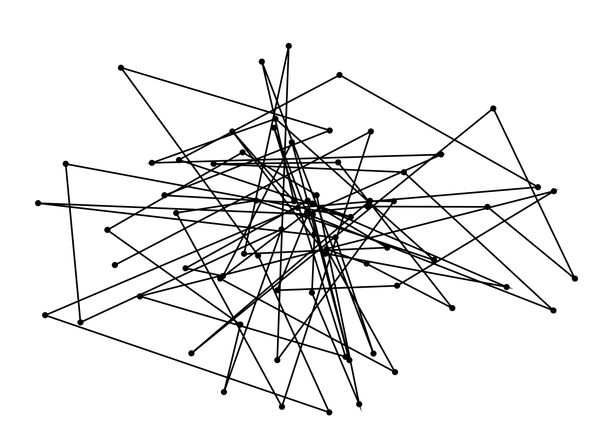
Experiments use two mobility models from BonnMotion [Asc⁺10], a Java mobility scenario generation tool:

1.

Random Walk [CBD02], based on the Brownian motion (mathematically described by Einstein in 1926 [SM01; Ein56]), where a node moves from its current location to a new location by randomly choosing a direction in the interval [0, 2π] and a speed between 0.1m/s and 1m/s, with a pause time of 10 seconds once the destination is reached. A representation of the Random Walk is given in 5.2.

2.

Truncated Lévy Walk [Rhe⁺11], which characterizes human mobility. Lévy walks are continuous-time random walks whose turning points are the visit points associated with the Lévy flights model. Parameters are a Levy exponent for flight length distribution α sets to 1, and a Levy exponent for pause time distribution β sets to 1. A representation of the Lévy Walk is given in 5.3.

Table of Contents