5.2 Centrality-Based Eventual Leader Election Algorithm

This section presents the Centrality-based Eventual Leader (CEL) election algorithm. In CEL, every node maintains a topological knowledge of the connected component to which it belongs. The algorithm builds this knowledge during node connections and disconnections (triggered by the cross-layer mechanism), and by sending knowledge messages to its neighbors. Nodes spread knowledge messages using probabilistic gossip, combined with a self-pruning mechanism that exploits the topological knowledge to reduce the number of messages sent. A new knowledge message is only sent after a connection or disconnection. Based on the component knowledge, the algorithm eventually elects one leader per component, which is placed at the center of the component.

5.2.1 Pseudo-code

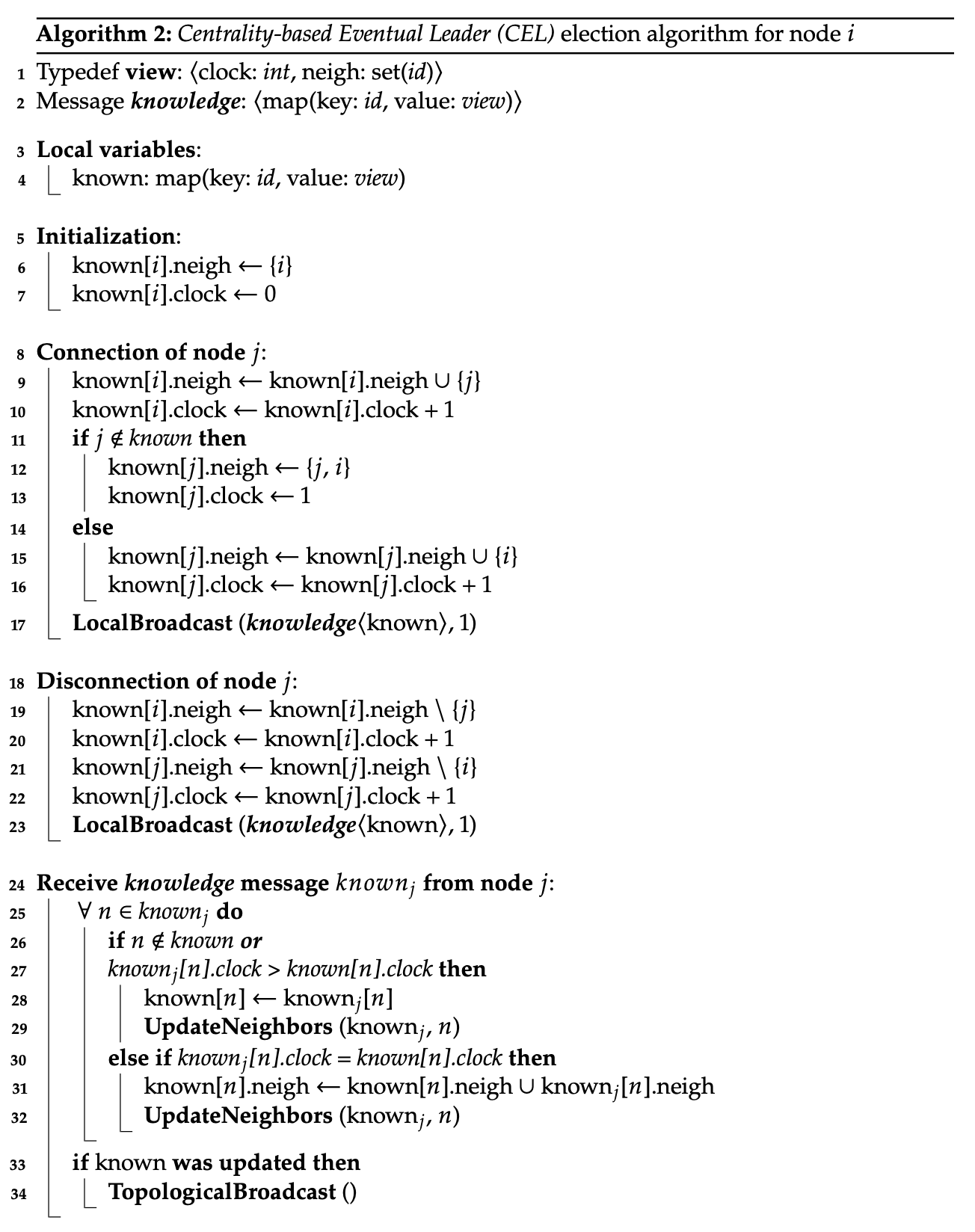
The pseudo-code of CEL for node i is given in Algorithm 2.

5.2.2 Data structures, messages, and variables (lines 1 to 4)

CEL uses a data structure called a view (line 1). A view associated to node i is composed of two elements:

1.

A logical clock value, acting as a timestamp and incremented at each connection and disconnection.

2.

A set of node identifiers, which are the current neighbors of i.

Each node i maintains a local variable (line 3) called known. This variable represents the current topological knowledge that i has of its current component (including itself). It is implemented as a map of view indexed by node identifier (line 4).

The only type of message exchanged between neighbors is the knowledge message (line 2). It contains the current topological knowledge that the sender node has of the network, i.e. its known variable.

5.2.3 Initialization (lines 5 to 7)

Firstly, node i initializes its known variable with its own identifier (i), and sets its logical clock to 0.

5.2.4 Node connection (lines 8 to 17)

When a new node j appears in the transmission range of i, the cross-layer mechanism of i detects j, and triggers the Connection method (line 8). Node j is added to the neighbors set of node i (line 9). As the knowledge of i has been updated, its logical clock is incremented (line 10).

Since links are assumed bidirectional, i.e. the emission range equals the reception range, if node i has no previous knowledge of j (line 11), the neighbor-aware mechanism adds both i and j in the set of neighbors of j (line 12). Then, i sets the clock value of j to 1 (line 13), as i was added to the knowledge of node j. On the other hand, if node i already has information about j (line 14), i is added to the neighbors of j (line 15), and the logical clock of node j is incremented (line 16).

Finally, by calling LocalBroadcast method (line 17), node i shares its knowledge with j and informs its neighborhood of its new neighbor j. Note that such a method sends a knowledge message to the neighbors of node i, with a gossip probability ρ, as seen in Section 2.8.0.0 [HHL02]. However, for the first hop, ρ is set to 1 to make sure that all neighbors of i will be aware of its new neighbor j. Note that the cross-layer mechanism of node j will also trigger its Connection method, and the respective steps will also be achieved on node j.

5.2.5 Node disconnection (lines 18 to 23)

When a node j disappears from the transmission range of node i, the cross-layer mechanism stops receiving beacon messages at the MAC level, and triggers the Disconnection method (line 18). Node j is then removed from the knowledge of node i (line 19), and its clock is incremented as its knowledge was modified (line 20). Then, the neighbor-aware mechanism assumes that node i will also disconnect from j. Therefore, i is removed from the neighborhood of j in the knowledge of node i, and the corresponding clock is incremented (lines 21- 22). Finally, node i broadcasts its updated knowledge to its neighbors (line 23).

5.2.6 Knowledge update (lines 24 to 34)

When node i receives a knowledge message known_j, from node j (line 24), it looks at each node n included in known_j (line 25). If n is an unknown node for i (line 26), or if n is known by node i and has a more recent clock value in known_j (line 27), the clock and neighbors of node n are updated in the knowledge of i (line 28).

Note that a clock value of n higher than the one currently known by node i (line 27) means that node n made some connections and/or disconnections of which node i is not aware. Then, the UpdateNeighbors method is called to update the knowledge of i regarding the neighbors of n (line 29). If the clock value of node n is identical to the one of both the knowledge of node i and known_j (line 30), the neighbor-aware mechanism merges the neighbors of node n from known_j with the known neighbors of n in the knowledge of i (line 31).

Remark that the clock of node n is not updated by the neighbor-aware mechanism, otherwise, n would not be able to override this view in the future with more recent information. The UpdateNeighbors method is then called (line 32). Finally, node i broadcasts its knowledge only if this latter was modified (lines 33-34).

5.2.7 Neighbors update (lines 35 to 41)

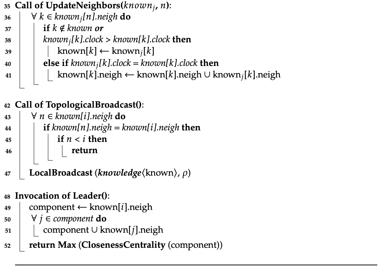
The UpdateNeighbors method (line 35) updates the knowledge of i with information about the neighbors of node n (line 36). If the neighbor k is an unknown node for i (line 37), or if k is known by i but has a more recent clock value in known_j (line 38), the clock and neighbors of node k are added or updated in the knowledge of node i (line 39). Otherwise, if the clock of node k is identical in the knowledge of node i and in known_j (line 40), the neighbor-aware mechanism merges the neighbors of node k in the knowledge of i (line 41).

5.2.8 Information propagation (lines 42 to 47)

The TopologicalBroadcast method (line 42) uses a self-pruning approach [LK01] to broadcast or not the updated knowledge of node i, after the reception of a knowledge from a neighbor j. To this end, node i checks whether each of its neighbors has the same neighborhood as itself (lines 43 to 44). In this case, node n is supposed to have also received the knowledge message from neighbor node j. Therefore, among the neighbors having the same neighborhood than i, only the one with the smallest identifier will broadcast the knowledge (line 45), with a gossip probability ρ (line 47). Note that this topological self-pruning mechanism reaches the same neighborhood as multiple broadcasts.

5.2.9 Leader election (lines 48 to 52)

The leader is elected when a process running on node i calls the Leader function (line 48). This function returns the most central leader in the component according the closeness centrality (line 52), as seen in Section 2.7, using the knowledge of node i. The closeness centrality is chosen instead of the betweenness centrality, because it is faster to compute and requires fewer computational steps, therefore consuming less energy from the mobile node batteries than the latter.

First, node i rebuilds its component according to its topological knowledge. To do so, it computes the entire set of reachable nodes, by adding neighbors, neighbors of its neighbors, and so on (lines 49 to 51). Then, it evaluates the shortest distance between each reachable node and the other ones, and computes the closeness centrality for each of them. Finally, it returns the node having the highest closeness value as the leader (line 52). The highest node identifier is used to break ties among identical centrality values. If all nodes of the component have the same topological knowledge, the Leader() function will return the same leader node when invoked. Otherwise, it may return different leader nodes. However, when the network topology stops changing, the algorithm ensures that all nodes of a component will eventually have the same topological knowledge and therefore, the Leader() function will return the same leader node for all of them [Ing⁺13].

Table of Contents