In the Topology Aware algorithm, every node keeps a topological knowledge of the connected component to which it belongs. The algorithm builds this component knowledge during node connections and disconnections (triggered by a probe system), and maintains it by sending either the full knowledge (called known) to new neighbors, or partial modifications (called updates) periodically to its neighbors.
The pseudo-code of the Topology Aware algorithm for a node i is given in Algorithm 4.2.1 and is described in the following.
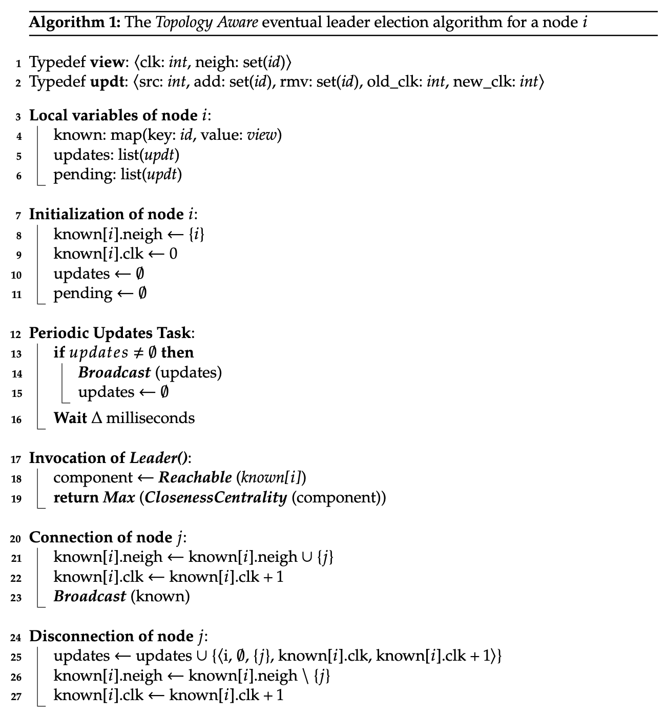
The two following data structures are used by node i:
Each node i maintains three local variables (line 3):
During communication, the variables known and updates are exchanged through two distinct types of messages identified by the name of the variables.
At the beginning, node i initializes its knowledge with its own identifier (i) and its logical clock set to 0.
Periodically, i.e. every Δ milliseconds, node i broadcasts its new updates list if not empty, and then set it to empty.
When a new node j appears in the transmission range of node i, it is detected thanks to the probe system and the Connection method is triggered (line 20). Node j is considered as a new neighbor and is added to the knowledge of node i (line 21). As the latter has been updated, the logical clock of node i is incremented (line 22).
Then, both nodes broadcast their current knowledge to share information about their component with each other, and also to inform neighbors about the new node. Therefore, node i broadcasts its known map (line 23) to its neighbors: node j then acquire topological knowledge about the component, while the other neighbors of i are informed about the new connection with j. Same process is executed by j in regard to node i and its neighbors.
When a certain number (γ) of probes from node j are not received by node i, node j is considered disconnected by i (line 24). An update structure is then created with the following information (line 25):
This tuple is added to the list of updates to be propagated later by the periodic updates task (line 12). Node j is then removed from the knowledge of node i (line 26) and the clock of node i is incremented (line 27).
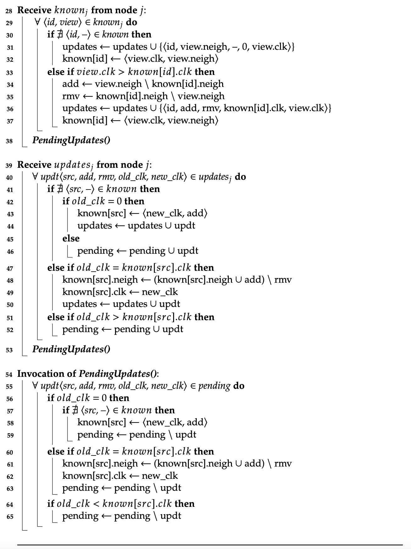
When node i receives the known map of node j (line 28), it checks each node id included in knownj (line 29). If id is a new node for it (line 30), node i creates an update containing the neighbors of node id with an old clock valued at 0, meaning that all neighbors of id are in the add set (line 31). The update is added to the list of updates to be propagated later by the periodic updates task. Then, the clock and neighbors of id are added to the knowledge of node i (line 32.
If id is known by i and the clock value of id is greater than the clock value known by node i for id (line 33), it means that id made some connections and/or disconnections of which node i is not aware. Hence, node i creates an update and computes the add set (line 34), which will be composed of the new neighbors for i that id informed in view, minus the neighbors of id which i already knew. The result represents new neighbors of id since its last received view. Then, node i computes the removed nodes of the update, by removing the received neighbors from the known neighbors of id (line 35), which represents disconnections since the last received view. The value of the old clock in the update is set to the clock value of id in the knowledge of node i, and the new clock value is set to the value of the received clock (line 36).
The update is added to the list of updates to be propagated later by the periodic updates task (line 12), and eventually, thanks to their previous knowledge and update exchanges, neighbors of node i will have the same knowledge as node i with identical clocks, thus, they will be able to apply this new update in their respective knowledge.
Finally, the clock value and neighbor identifiers of id are added to the knowledge of i (line 37) and the PendingUpdates method is called to apply previously received updates (line 38).
When node i receives updates from node j (line 39), each update adds or removes neighbors of a source node src (line 40). Following the old clock value, an update can be applied, saved in the pending list to be applied later, or discarded.
If the old clock is equal to 0 (line 42), the update contains all the neighbors of node src (see Knowledge reception paragraph), and the update is applied (line 43) if node i does not have any information about node src (line 41). If the old clock is equal to the clock of node src in the current knowledge of node i (line 47), the update corresponds to new information. The update is then applied, i.e. neighbors are updated (line 48) as well as the clock (line 49). In both cases, the updates are added to the updates set of node i (lines 44 and 50), to be propagated later to neighbors through the periodic updates task.
Note that an update cannot be applied when it is more recent than other updates not yet received by i, which should have been applied before the former. This out-of-order update receptions might happen if the component contains cycles, i.e. when the old clock is greater than the clock of src in the knowledge of i (line 51), or when node i does not have any information about node src and the old clock is greater than 0 (line 45). In those cases, node i saves the update in a pending updates list (lines 46 and 52), and will try to apply it in the future, after new updates will be received (line 53).
PendingUpdates (line 54) checks the updates that can be applied from the pending list (line 55). To reduce message exchanges and improve performance, updates that cannot be applied when first received are saved, and the algorithm tries to apply them after new information is received.
When an update is applied (i.e. the knowledge of i changes, lines 58 and 61-62), the latter is removed from the pending list (lines 59 and 63). If the clock value of the current knowledge is greater than the old clock value of the update (line 64), the update is also removed for the pending list (line 65), meaning that node i receives a knowledge or updates from a node with more recent information.
When a process running on node i requires a leader, it calls the local Leader method (line 17) which computes and returns, based on the knowledge of i, the best leader according to the closeness centrality (line 19). The closeness centrality defined in Section 2.7 is used rather than the betweenness centrality, because it is computed faster and requires fewer computational steps, so use less energy from the mobile nodes. In order to compute the closeness centrality, node i, starting from itself, get the set of reachable nodes according to its topological knowledge of the component (line 18). Then, for each reachable node, it computes the shortest distance between this node and the other reachable ones, obtains the closeness centrality, and deduces the most central node as the leader (line 19). The highest node identifier is used to break ties among identical centrality values.
If all nodes of the component have the same knowledge of the topology, the Leader() call returns the same leader node to all of them. Otherwise, it may return different leaders for distinct nodes. However, if topology changes cease, the algorithm ensures that all nodes of a connected component will eventually have the same topology knowledge and, therefore, will have the same leader node [Ing+13].
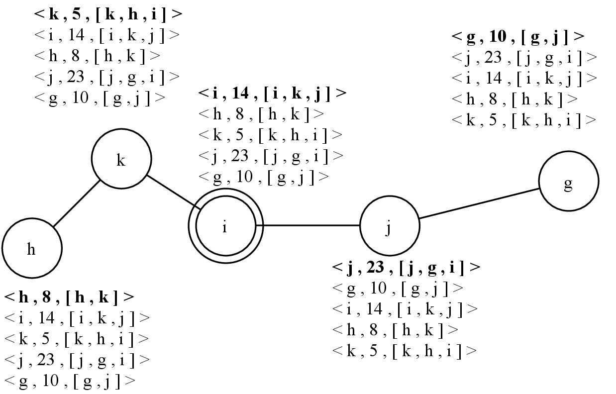
This section presents examples of the execution of Topology Aware algorithm, showing the connection between node i and node j.
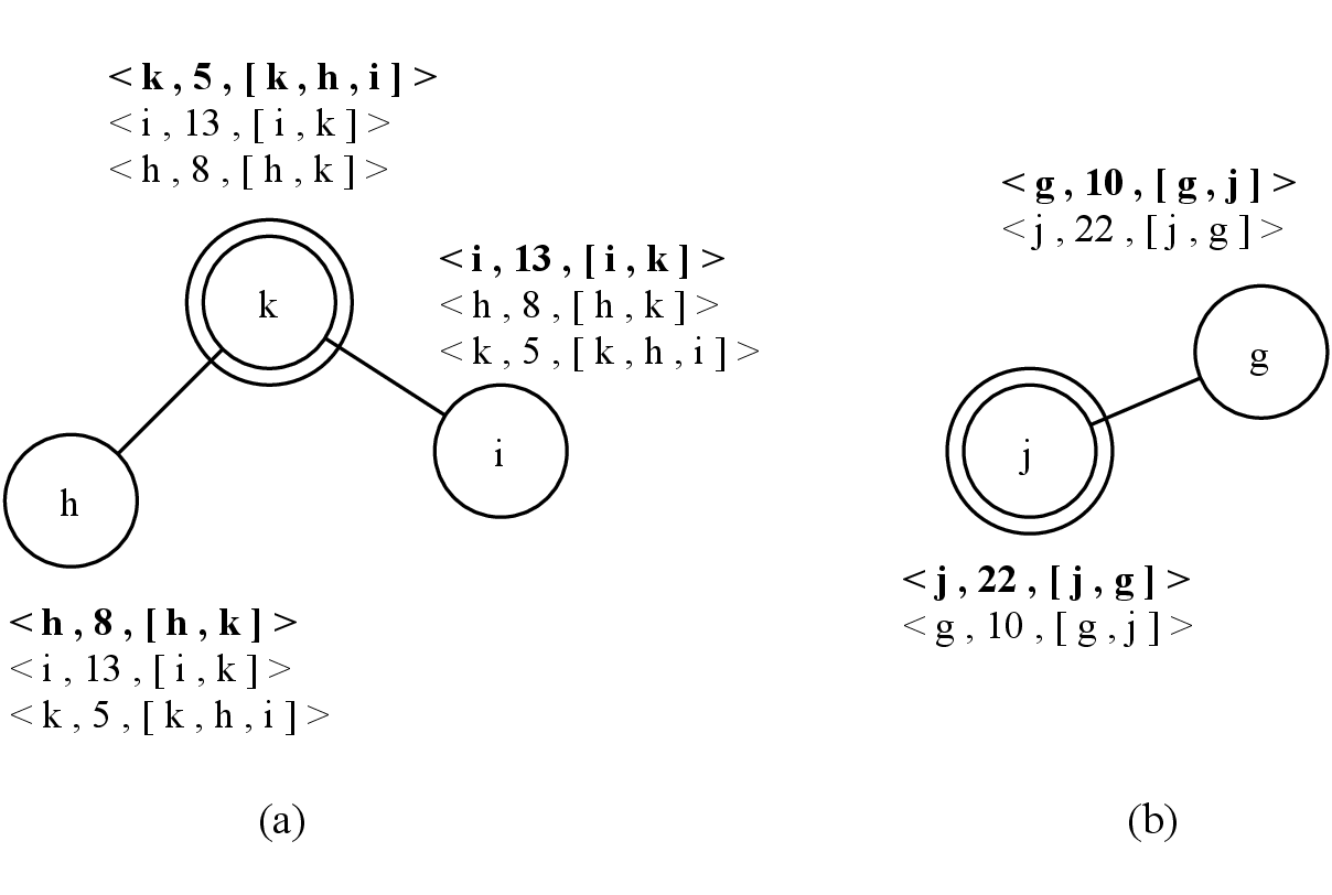
Initially, in 4.1, the system is composed of two connected components: nodes h, i, and k in 4.1.a, and nodes j and g in 4.1.b. Each node has its own knowledge composed of identifier,clock,set(neighbors) /span>, with arbitrary initial values used for the sake of the example. One leader is currently elected per component, respectively nodes k and j. Nodes j and g have the same closeness centrality, therefore, the highest node identifier is used to break the tie, as presented in Section 4.2.10, and since g <j, node j is the leader.
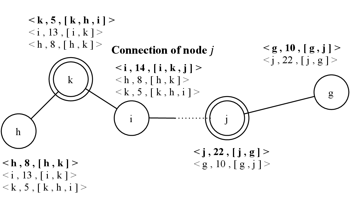
In 4.2, the underlying probe system of node i first detects node j and triggers the Connection method described in Section 4.2.5. Therefore, node i adds node j in its neighbors list, and increments by one its clock value, previously sets to 13.
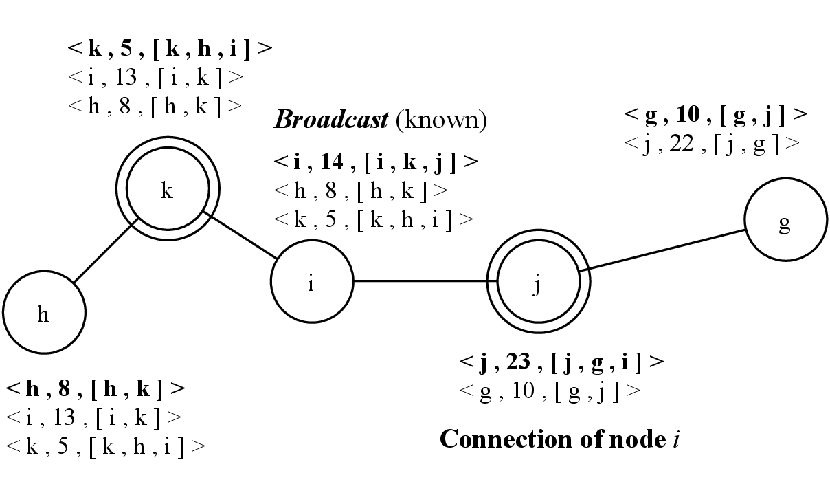
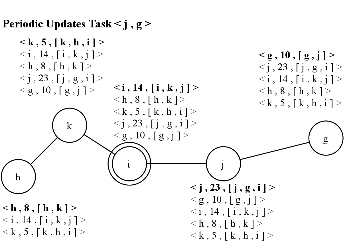
Then, in 4.3, node i broadcasts its knowledge in order to share its view of the network with node j. Meanwhile, the probe system of node j has detected node i and triggers the Connection method of node j. Node i is added to the neighbor list of node j and the latter increments its clock value from 22 to 23.
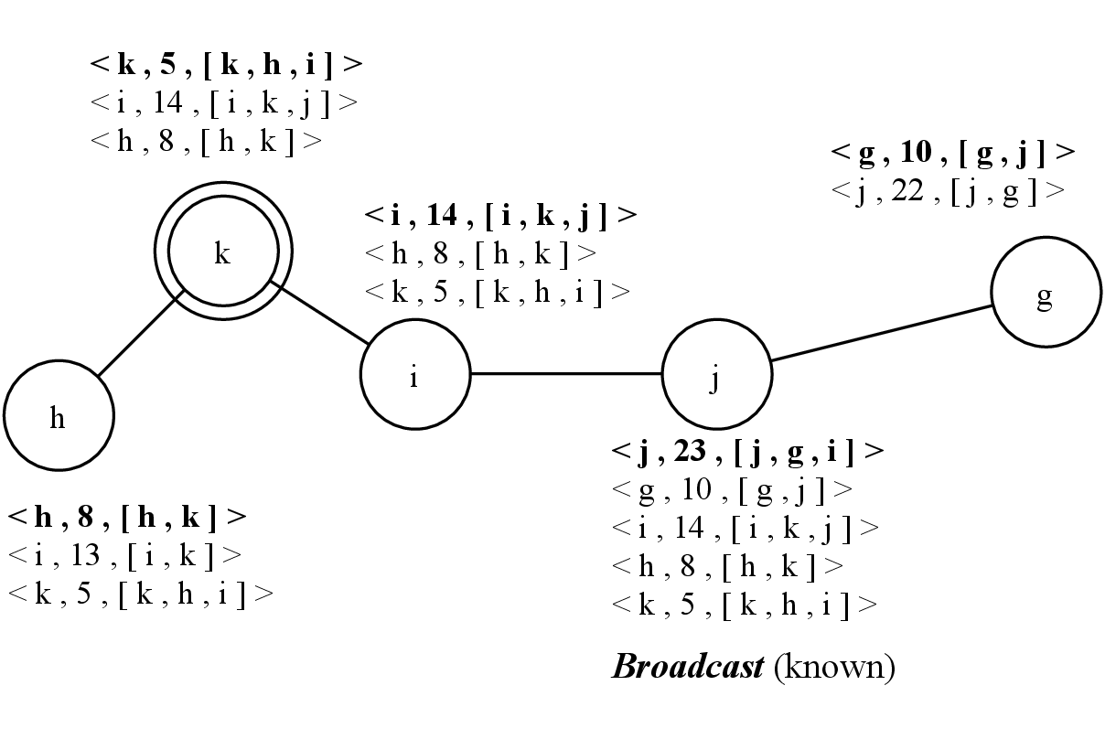
In 4.4, node j broadcasts its knowledge to complete the Connection method, and it receives a knowledge from node i. According to this new knowledge, node j is not the leader anymore. Since node j received a knowledge from node i, it creates an update. However, in this case, the update will not be usefull since its neighbors already received its knowledge. Note that node k also received the knowledge of node i, therefore, it follows the steps described in Section 4.2.7: the received clock of node i is higher than the known clock of i in the knowledge of node k (14 13, line 33), meaning that new information is received. Therefore, node k updates the entry of node i in its knowledge by adding node j as a new neighbor and updating the clock of node i from 13 to 14. It also creates an update i,add(j),rmv(−),13,14 that will be sent by the Periodic Updates Task.
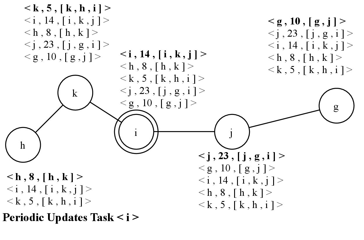
Then, in 4.5, nodes i and g receive a knowledge from node j. Both nodes update their knowledge and create updates with the new received information, that will be broadcast later. According to this new knowledge, node i considers itself as the leader since it has the highest closeness centrality.
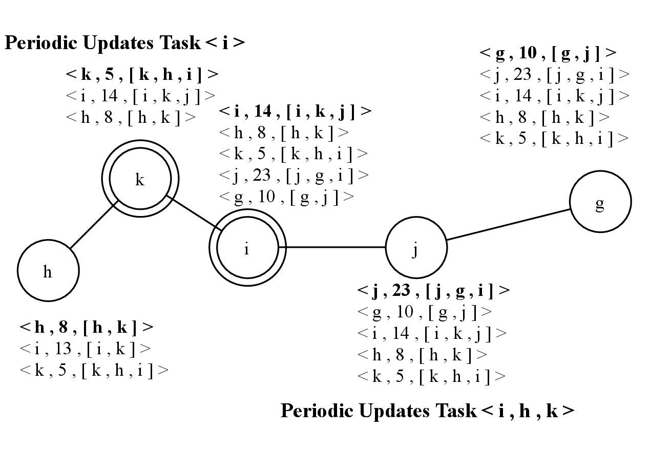
In 4.6, the Periodic Updates Task of both nodes i and g send their update. Node h received the update of node k and updates the entry of node i in its knowledge with the more recent information received. Therefore, it creates an update with the new information received, that will be sent later.
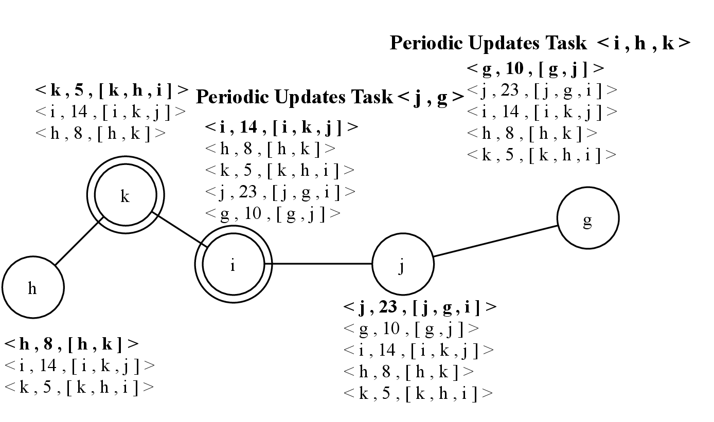
Then, in 4.7, node k received the update sent by node i, with information about nodes j and g. Thus, it updates its knowledge and creates an update containing this new received information. The Periodic Updates Task of node h sends the update with information about node i.
In 4.8, the Periodic Updates Task of node k sends the update with information about nodes j and g.
Finally, in 4.9, node h receives the update from node k with information about nodes j and g. It updates its knowledge and creates an update with the new received information, that will be sent later by the Periodic Updates Task (not shown in the example). All nodes have the same knowledge of the component. Hence, the invocation of Leader() method of Ω failure detectors returns the most central node according to the closeness centrality: node i, which is the leader.